See this paper
\documentclass{article}
\usepackage{tikz}
\pagestyle{empty}
\begin{document}
\begin{center}
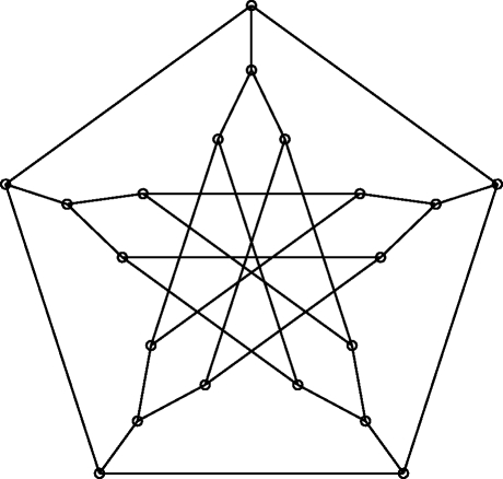
\begin{tikzpicture}[style=thick]
\foreach \x in {18,90,...,306}
{
\draw (\x:4cm) circle (2pt) -- (\x+72:4cm);
\draw (\x:4cm) -- (\x:3cm) circle (2pt);
\draw (\x:3cm) -- (\x+15:2cm) circle (2pt);
\draw (\x:3cm) -- (\x-15:2cm) circle (2pt);
\draw (\x+15:2cm) -- (\x+144-15:2cm);
\draw (\x-15:2cm) -- (\x+144+15:2cm);
}
\end{tikzpicture}
\end{center}
\end{document}